In my post, Harmful Algal Blooms – Part 2, I wrote about the challenges involved in monitoring harmful algal blooms (HABs). I also wrote about working with NASA DEVELOP last summer to develop a method to track harmful algal blooms using remote sensing data. We hoped to develop a tool that would allow HAB researchers to quickly identify algal hotspots.

One of our big challenges was finding dates for which there was both good satellite data and good ground data. We found one such date, July 3, in 2013.

Why only one day? NASA’s MODIS Aqua satellite monitors the Chesapeake Bay on a daily basis. But, Landsat covers the area only once every 16 days. If that day is cloudy, there might be very little overlap between the Landsat and MODIS Aqua images.

Here is a Landsat true color image for Path 13, Row 34 for June 17, 2013 downloaded from USGS’s EarthExplorer website:

Here is the MODIS image for the same day:

As you can see, having plenty of satellite imagery doesn’t mean that we have good data about conditions in the Chesapeake Bay. And, unfortunately this happens a lot. What we really needed to  complete our project was a Golden Day: a day with clear skies where there was a boat cruise and Landsat coverage in addition to daily MODIS Aqua data. A Golden Day like that would allow us to verify the model.

The “Golden Day of Data Collection” occurred on August 17, 2015. On that day, there was a large bloom of Alexandrium monilatum in the York River and a possible bloom of Cochlodinium polykrikoides on the James River. As Landsat 8 passed above the Alexandrium bloom, the Virginia Institute of Marine Science used a boat to monitor chlorophyll in the water.  You can see the boat path (red squiggle) on the Landsat image below.  

The MODIS Aqua imagery for the same day shows high levels of Chlorophyll in the Chesapeake Bay and its tributaries:

Since our term with DEVELOP was over, the “Golden Day of Data Collection” didn’t help our project. However, the new team received plenty of information to verify our work. You can learn about their work  here.

Hyperspectral Data

But, the story doesn’t end with good verification data. One of my frustrations with working with Landsat data was that Landsat 8 is multispectral. It’s sensors measure 11 bands of reflectance ranging from 0.43 to 12.51 micrometers. But, these are wide bands and many species of bioluminescent phytoplankton like Alexandrium monilatum and Cochlodinium polykrikoides emit, absorb, and reflect light in very narrow ranges of  wavelengths.

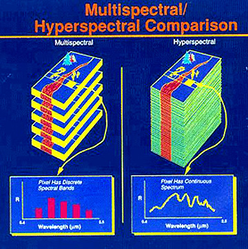
While multispectral sensor bands are wide, hyperspectral sensors divide the same range of wavelengths into dozens, hundreds or even thousands of much thinner slices or bands. This image from Wikipedia explains the concept visually:

On the Golden Day, a NASA test flight equipped with a hyperspectral sensor passed overhead and obtained hyperspectral imagery of the area. The sensor was able to measure 283 bands of reflectance ranging from .35 to 10.50 micrometers. This means that the sensor could measure the very specific wavelengths I was interested in.

The true color images look like this:

 

A pixel in this image is about 2 meters by 3 meters.

Because the images show water from a high altitude, they aren’t at all very exciting too look at. However, having this type data  was very exciting to me. I volunteered to work with the hyperspectral data during the fall term. This work is my project for GIS 255 and GIS 295 and I will describe my project (and the frustrations of working with the hyperspectral data) in future posts.

Go to: Harmful Algal Blooms, Part 4: What is a Spectral Signature?